How To Enhance Your Spreadsheets With Excel Font Color Formula

Excel is one of the world’s most widely used spreadsheet programs and for a good reason. It’s powerful, versatile, and allows users to manipulate data seemingly endless ways.

One of the most important features of Excel is its ability to apply formulas to cell data, making it easy to analyze and manipulate large amounts of information quickly. One such formula that can be incredibly useful in enhancing your spreadsheets is the font color formula.

Using this formula, you can automatically change the color of the text in your spreadsheet based on certain conditions or criteria. This can make it much easier to quickly identify important data, highlight trends, or draw attention to specific information. We’ll walk you through the steps to using the excel font color formula, from setting up the formula to applying it to your data.

What Is A Font Color Formula In Excel?

A font color formula in Excel can change the text colour based on specific conditions or criteria. It allows you to automatically apply different colors to cells or ranges of cells depending on the values they contain. This can be useful for highlighting important information, creating visual cues, or organizing and categorizing data.

The font color formula in Excel typically involves using conditional formatting rules that specify the conditions for applying different colors and the corresponding formulas or criteria to evaluate. By utilizing font color formulas, you can make your spreadsheets more visually appealing and easier to interpret.

How To Use Font Color Formula In Excel?

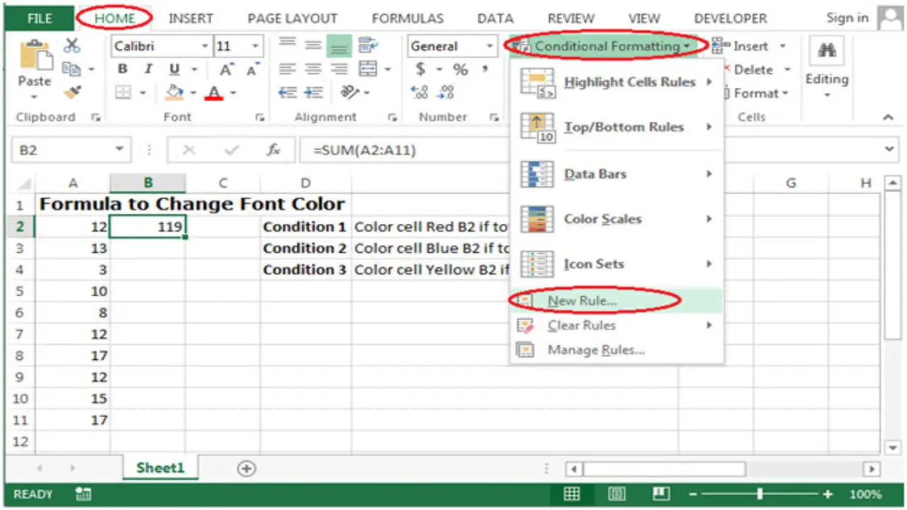
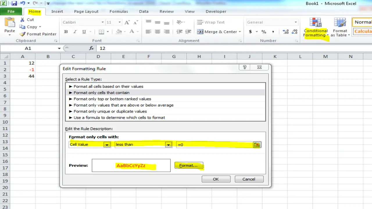
Using a font color formula in Excel can be useful to enhance your spreadsheets and make certain data stand out visually. To use the font color formula, you must select the cell or range of cells to which you want to apply the formatting. Then, go to the “Home” tab and click on the “Conditional Formatting” option in the “Styles” group.

Choose “New Rule” from there and “Use a formula to determine which cells to format.” In the formula box, enter the condition you want to apply, such as “=A1>100” for cells with a value greater than 100. Next, click the “Format” button and choose the desired font color from the options provided. Finally, click “OK” to apply the font color formula formatting to your selected cells.

Enhance Your Spreadsheets With Excel Font Color Formula

Enhancing your spreadsheets with the Excel font color formula can add a visual element to your data and make it easier to interpret. The font color formula allows you to change the color of text based on specific conditions or criteria. For example, you can use the formula to highlight cells that contain certain values or meet certain criteria.

This can be particularly useful when working with large datasets or complex formulas, as it allows you to quickly identify and analyze important information. By utilizing the font color formula in Excel, you can create visually appealing and informative spreadsheets that effectively convey your data.

Using Font Color Formula For Data Analysis

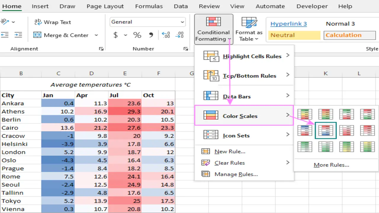
Using font color formulas in Excel can be a powerful tool for data analysis. You can quickly and visually identify patterns, trends, or outliers by assigning specific colors to different values or conditions in your data. For example, you can use conditional formatting to highlight cells that meet certain criteria, such as all sales above a certain threshold or all overdue tasks.

This can make it easier to spot important information at a glance and make data-driven decisions. By using font color formulas effectively, you can enhance the readability and interpretation of your data in Excel.

Customizing Font Color Formula With Additional Conditions

Customizing the font color formula in Excel allows you to enhance further and personalize your spreadsheets. You can create more specific and targeted formatting rules by incorporating additional conditions. With the font color formula, you can highlight cells that meet specific criteria or contain certain values.

This flexibility gives you greater control over your data’s visual appearance and readability. Use Excel’s font color formula to create customized and visually appealing spreadsheets catering to your unique needs. Excel, conditional formatting, personalized formatting rules, customize, visual appearance, readability, data analysis.

How To Change The Font Color Of A Cell In Excel

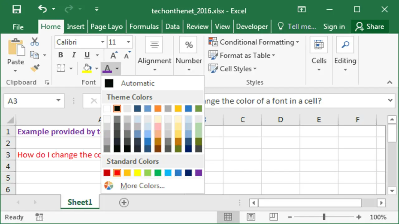
Changing the font color of a cell in Excel is a simple process that can help make your spreadsheet more visually appealing and easier to read. To change a cell’s font colour, select the cell or cells you want to modify. Then, go to the “Home” tab on the Excel ribbon and locate the “Font” section. In this section, you will find a small icon with an “A” and a paint bucket next to it.

Click on this icon to open the font color menu. From here, you can choose from a variety of predefined colors or select “More Colors” to choose a custom color. Once you have selected your desired font color, click “OK” to apply the change.

Conclusion

Using Excel font color formula can enhance the visual appeal of your spreadsheets and make it easier to analyze and interpret data. By applying font color formulas, you can highlight specific data points, identify trends or patterns, and draw attention to important information.

It’s important to remember that font color formulas should be used judiciously and with a clear purpose in mind. They should complement the overall design and readability of your spreadsheet. Furthermore, the flexibility of the formula allows for customization and creativity in your spreadsheet design. Utilizing this feature can save time and increase efficiency, making your work stand out professionally.

Frequently Asked Questions

1.How Do I Color Text In Excel Formula?

Ans: To color text in Excel using a formula, apply the “Conditional Formatting” feature. Select the cells or range, go to the “Home” tab > “Conditional Formatting” > “New Rule.” In the dialogue box, choose “Use a formula to determine which cells to format.” Enter your TRUE/FALSE formula and define the formatting condition. Finally, select the desired font color and other formatting options.

2.Can Excel Formula Detect Font Color?

Ans: No, Excel formulas cannot directly detect font color. However, you can use conditional formatting to highlight cells based on font color. This feature lets you set up rules that change the cell’s format based on its value or other criteria, allowing for dynamic and visually appealing spreadsheets.

3.What Is The Formula For Red Font In Excel?

Ans: To apply red font color in Excel, use the formula “=IF(logical_test, “red”, “)”. Replace “logical_test” with your condition. If the condition is true, the font will turn red. Remember to enclose “red” in double quotes to specify the color.

4.How Do I Change The Font Color In The Formula Bar In Excel?

Ans: Unfortunately, it is not possible to change the font color in the formula bar in Excel. The text in the formula bar will always appear in black. However, you can change the font color of cells or ranges using conditional formatting or cell formatting options. If you need to apply different formatting to a specific result, you can use IF or conditional statements within the formula.

5.How Do I Apply Font Color Formulas In Excel?

Ans: To apply font color formulas in Excel, use the “Conditional Formatting” feature. Select the desired cells, navigate to the “Home” tab, click on “Conditional Formatting,” and choose “New Rule.” In the dialogue box, enter your formula and select the desired font color and formatting options. Finally, click “OK” to apply the formula.